Learning Monte Carlo Methods Poorly: Randomly Find π by Throwing Yard Darts

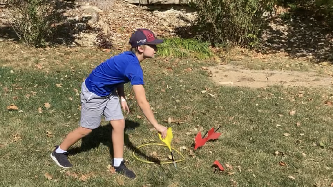
(Originally posted on LinkedIn)

Monte Carlo is a way to solve a problem by randomly throwing crap at it until it works. If you know me, you know this is my favorite way to do things. So, when I heard there was a broad class of computational algorithms that did this formally, I was smitten. Still am. Ok, so, what does that mean? Basically, you have a complex problem that is impossible to solve because there’s some unknown variables, or there’s unquantifiable risk (my faaaaavorite) you can plug your problem into a system that uses randomness to zone in on an approximate solution. Usually that solution is probabilistic so you wind up with a mean and a variance so you can have a good idea of how close your result is to the actual number. Or, in other words, you get a solution that is close enough for Jazz. How about a bad example for fun? Let’s say you want to know how much pizza you need for your weekly yard darts tournament. If that pizza was square, you could figure out the area easily by multiplying the sides. But, pizza is round so that’s not going to work. So, you draw a picture:

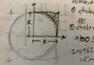
You realize you can fit your pizza inside a square and it seems like there’s a consistent relationship between the area of the square and that circle inside of it… What if there was a factor, or some sort of constant you could apply to the easy thing to get the hard thing? You’re thinking about darts so…. What if you randomly threw darts at it? Most would wind up inside the circle, but some would wind up outside that circle… Can that give you the proportion you need? Something like:

area of the square * Number of darts inside circle / total darts = area of a circle

And, if you think about it, the more darts you throw, the better your estimate should be…. So, instead of doing this in the back yard with jarts, you whip up a quick little program:

i=1
n<-10000
result = array( dim=c(3,n))

for (i in 1:n) {

  hits <- data.frame(x=runif(i,-1,1),y=runif(i,-1,1))
  hits$d<-sqrt(hits$x^2+hits$y^2)

  inside <-subset(hits, d<1)

  estpi<-4*nrow(inside)/i

  esterr<-pi - estpi

  result[1,i]<-i
  result[2,i]<-estpi
  result[3,i]<-esterr
}
# plot 
hits$col<-ifelse(hits$d > 1, 1,2)
plot(hits$x,hits$y, col=c('red','blue')[hits$col],pch='.') 1

This is assuming you’re doing just 1/4 of the circle (like the hand drawn picture above) which is why I’m multiplying the estimate by 4. Anyway, the plot of throws looks like this:

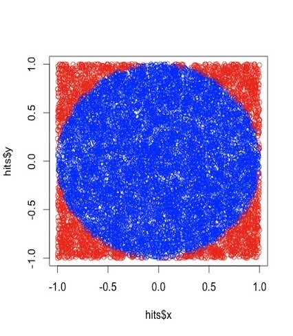
When I ran that, it said the proportion was 3.096… (spoiler, it should be 3.14) but that was for 1,000 throws. What if I do 5k? 10k? Will the value get closer to 3.14? Let’s see. Let’s try 1 throw, then 2, then 3 all the way to 10000 a bunch of times each and see if our estimates get better by plotting the errors on a scatterplot.

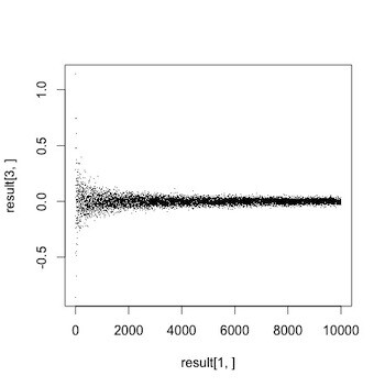
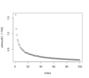
Look at that graph, how do we really know that error is going to zero? I don’t think we do. I’d like to try something a little different. Re-run the first program (where dart throws = 1000) a few times. Notice how you get a different estimate each time. It might be nice to run that program a thousand times and see what the result’s distribution looks like. Namely, it would be nice to know the accuracy’s standard deviation for the 1,000 runs. That should illustrate the result’s consistency that particular number of dart throws. I’d argue that more dart throws not only gives us a result that’s more accurate (error closer to zero), but also a result that is more consistent (smaller standard deviation). Could we write a program that calculates standard deviation of results for 1 throw, then 2, then 3 all the way up to 1000 and graph the results? Sure. Here’s one way to do exactly that:

runs<-1000 #number of runs per test 
tests<-1000 #number of tests. test 1 throws 1 dart, 2 throws 2 darts, etc.
sdresult = array(dim=c(1,tests))

test=1
for(test in 1:tests){

  i=1
  result = array( dim=c(3,runs))

  for (i in 1:runs) {
    hits <- data.frame(x=runif(test,-1,1),y=runif(test,-1,1))
    hits$d<-sqrt(hits$x^2+hits$y^2)
    inside <-subset(hits, d<1)
    estpi<-4*nrow(inside)/test
    esterr<-pi - estpi

    result[1,i]<-i
    result[2,i]<-estpi
    result[3,i]<-esterr
  }
  sdresult[1,test]<-sd(result[3,])
}
plot (sdresult[1,])t

Here’s the standard deviation plot of the error for 1 to 100 dart throws. Y axis is standard deviation of error, X is number of throws:

Here’s the standard deviation for 1 to 1000 dart throws:

We already showed that the more throws gives you more accurate results. This graph shows that more throws also gives a smaller variance in those results. This graph nicely illustrates the non-linear relationship between accuracy and number of trials. You get a big boost of accuracy going from 10-20 throws, but not a whole lot going from 600 to 1000.

Ok, so what did we do here? We estimated the mystical number π by throwing a bunch of yard darts at a target. We showed that the estimate we calculated is close and we showed that we could sort of quantify our accuracy based on how many random throws we did.

Is this Monte Carlo? Well… loosely… If it seems interesting to you, go to wikipedia and find some youtube explainers to learn more. It is part of a family of fantastic, powerful methods that can be a lot of fun and very useful.

Finally… I want to come clean, I did the programs a long time ago (I don’t remember anything about R anymore….) and wrote something similar up on a different site. So, if you’ve seen this before (doubtful) maybe that’s why. I also go the idea of finding pi by throwing darts from some online MIT math class I followed. So, not my idea, but still a lot of fun. Lastly, Jarts are dangerous and should not be played with… but, if you’re up for a game, let me know.